TurboQuant: The Compression Shannon Would Approve

TurboQuant (TQ) solves the biggest bottleneck in modern AI search: memory efficiency. As embedding models become larger, storing high-dimensional vectors in RAM becomes a cost-prohibitive challenge. While traditional quantization methods can reduce storage, they often sacrifice too much accuracy (recall). TurboQuant acts as a strategic bridge, it provides the blazing-fast setup speeds of simple compression while hitting the high-precision recall levels previously reserved for slow-to-train algorithms

TurboQuant is a high performance online vector quantization (VQ) framework engineered for near-optimal distortion rates in high dimensional vector retrieval, designed to solve a classic AI challenge “ how do you search through millions of complex high dimensional vectors without exhausting your server’s memory?

Theoretical foundation of TQ

how much information can be compressed without losing too much meaning ?

this question was established by the father of information theory Claude Shannon, imagine sending a large file over a slow connection, Shannon basically states that there is a mathematical limit to how much you can compress that file without losing information(distortion)

if you try to compress data below its entropy( its information content ) you lose data
if you stay above that limit you can reconstruct the original data almost perfectly

TQ uses Shannon’s principle to decide “how many bits do i need to represent this vector so that, when i decompress it later, it is still mathematically close to the original?”.

[Image below] Shannon’s Source Coding Theorem: This establishes the mathematical floor, the minimum bits required to represent data without losing its essential geometric structure

Claude Shannon’s work is the ‘physics’ of data. It tells us there is a mathematical limit to how much we can shrink a file before the information becomes distorted. TQ is special because it is engineered to get as close to this theoretical limit as possible. By rotating vectors to induce a concentrated Beta distribution, TQ allows us to apply optimal scalar quantizers per coordinate, ensuring that we minimize distortion while keeping our storage footprint tiny

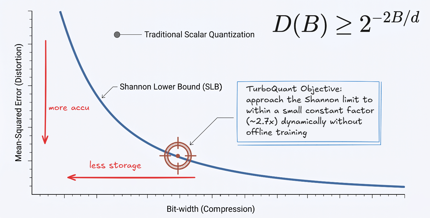
looking at the image above what we want is Minimum bit-width : to save storage and RAM , and we want Minimum distortion (MSE) to keep high search accuracy (just follow the red arrows) and the what TQ want to find is the sweet spot on the curve where minimizing distortion while keeping the bit-width as low as possible

The SLB in the image refers to the mathematical floor of distortion, meaning when you compress a vector you must lose some information for that the SLB is a formal proof that identifies the minimum possible distortion for any given bit-width, it tells you “no matter how smart the quantization algorithm is, you cannot possibly compress this data better than this specific limit”

The goal is to eliminate the memory overhead of traditional vector quantization while maintaining near optimal distortion rates. instead of adapting the grid to the data, rotate the data to fit a fixed mathematical grid

How TQ works (the rotation trick)

TurboQuant doesn’t just cut corners. It first uses a Walsh-Hadamard rotation to transform the input vectors. This ‘smooths’ the data, creating a distribution that is perfect for the Lloyd-Max quantization algorithm to work on. Because this happens on-the-fly, we avoid the need for expensive, offline training phases that other algorithms require

in high dimensions, a random rotation spreads energy across all coordinates (rotation preserves all dot products)

$R\vec{x} \cdot R\vec{y} = \vec{x} \cdot \vec{y}$

this is what makes the whole thing safe. rotating the vectors doesn’t destroy their geometric relationships, L2 distances and angles stay exactly the same. you’re just changing the coordinate system, not the meaning

step 1 : Inducing the beta distribution :

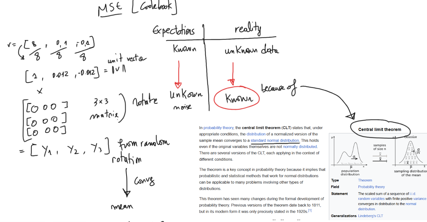
this step consist of applying a fast random orthogonal rotation (walsh-hadamard transform) to every vector. every coordinate now approximates a standard normal distribution $X\sim\mathcal{N}\left(0,\frac{1}{d}\right)$

because the shape is highly predictable we no longer need to calculate and store costly normalization data for every block

we show why rotation works when you rotate a vector using the Hadamard transform, each coordinate starts to follow a bell curve (normal distribution), this is the central limit theorem in action, because we know the shape in advance we don’t need to learn anything from the data. the codebook (the fixed lookup table) can be precomputed once and reused forever

step 2: optimal scalar quantization:

with data evenly distributed we apply a fixed lookup table (lloyd-max codebook) to each coordinate independently (the codebook is a single 16-level codebook (for 4-bit) is used for the entire dataset)

any pair of stored vectors can be stored against each other directly from their indices, requiring zero floating point reconstruction

step 3: Erasing Inner product Bias

the problem is that MSE optimal quantizers are mathematically biased for inner-product estimation, here TurboQuant applies the quantized Johnson-lindenstrauss 5QJL) algorithm to the tiny residual error left over from the first stage

the result is that each coordinate of the residual is reduced to a single but (+1 or -1) which eliminates bias and results in a perfectly unbiased inner product quantizer

So where does TurboQuant actually sit compared to every other method? The table below shows all the options:

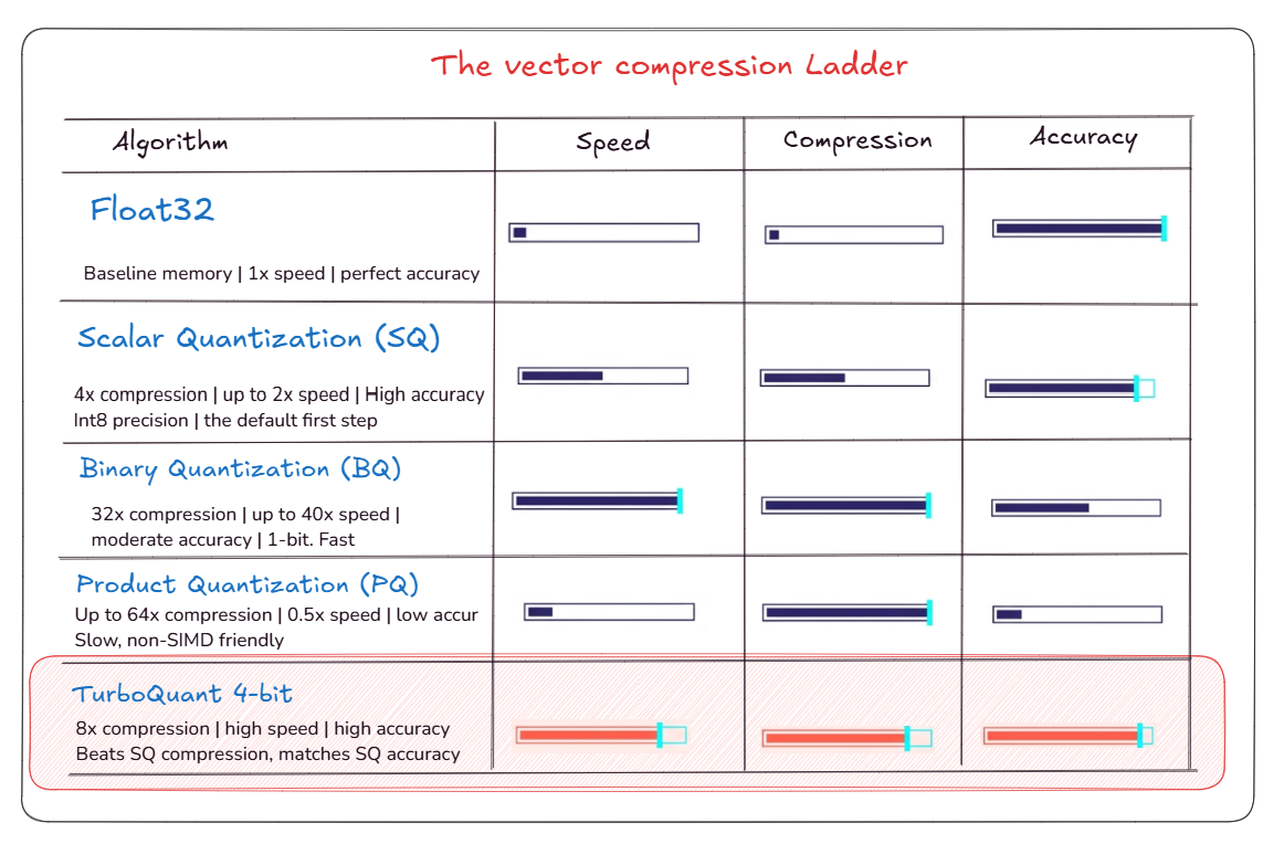
TQ 4-bit hits the sweet spot: it compresses 8x (twice as much as Scalar Quantization) while keeping accuracy almost identical. Unlike Product Quantization which is slow and inaccurate, TQ is fast AND accurate. It’s the only method in the table that beats SQ on compression without sacrificing recall

Reminder of metrics

Manhattan Distance (L1)

The one that breaks under TurboQuant’s rotation because it measures distance in a grid-like path.

$D_{L1}(\mathbf{x}, \mathbf{y}) = \sum_{i=1}^{n} |x_i - y_i|$

Euclidean Distance (L2)

The standard straight-line distance between two points. TurboQuant preserves this perfectly.

$D_{L2}(\mathbf{x}, \mathbf{y}) = \sqrt{\sum_{i=1}^{n} (x_i - y_i)^2}$

Dot Product (Inner Product)

Measures how aligned two vectors are, scaled by their magnitude. Highly optimized in vector databases.

$\mathbf{x} \cdot \mathbf{y} = \sum_{i=1}^{n} x_i y_i$

Cosine Similarity

Measures the angle between two vectors, regardless of their length (magnitude). It’s essentially the Dot Product of normalized vectors.

$\text{Cosine}(\mathbf{x}, \mathbf{y}) = \frac{\mathbf{x} \cdot \mathbf{y}}{|\mathbf{x}| |\mathbf{y}|} = \frac{\sum_{i=1}^{n} x_i y_i}{\sqrt{\sum_{i=1}^{n} x_i^2} \sqrt{\sum_{i=1}^{n} y_i^2}}$

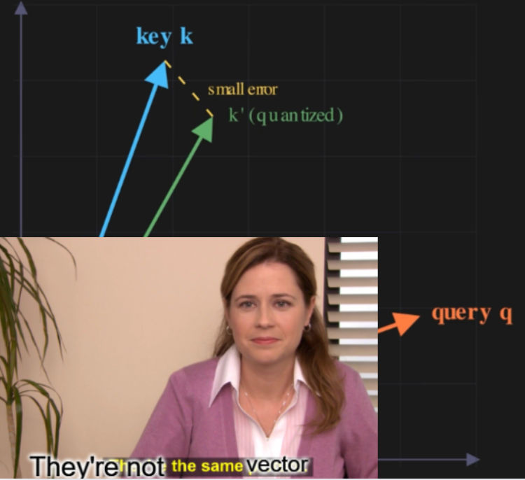
Now that we know how vectors are compared, here’s why compressing them is tricky:

here’s the core problem with quantization. When you compress a vector, you get back something slightly different, not the original. The key (stored vector) and the query (search vector) are NOT the same thing anymore. This is called the quantization error, and it’s what causes wrong search results

the image below shows this visually. The yellow bars are the original vector values, the green bars are what we stored after compression, and the blue/red bars are the error, the difference between them. TQ’s entire job is to make those error bars as small as possible

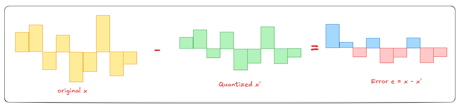
this error is unavoidable, you always lose something when you compress. the question is HOW MUCH you lose, and whether that loss changes the final search ranking. TQ uses the two-stage pipeline (rotation + scalar quantization + JL correction) to keep this error as mathematically small as possible

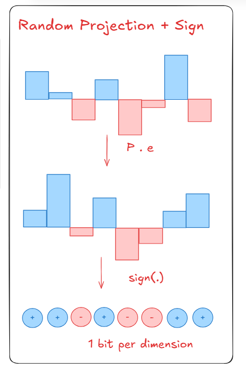
the diagram above shows Step 3. The residual error vector (the leftover after Step 2) gets randomly projected (P) , and then only its SIGN (+1 or -1) is kept, 1 bit per dimension. you might think this is like throwing away information, but it’s mathematically proven to fix the inner product bias completely as the QJL paper mentioned that with just the sign information, it allows you to recover an unbiased estimate of dot products

One limitation worth knowing: L1 distance

TurboQuant require full reconstruction for L1 ? :this is because of the core math of how TQ works

to compress vectors so efficiently TQ as we mentioned applies a random orthogonal rotation (a randomized Hadamard transform) to the vectors before quantizing them

what rotation preserves : rotating a shape doesn’t change straight line distances between points (L2) or the angles between them (cosine)

because rotation breaks L1 math you cannot compute L1 distance while the vector is in its TQ compressed/rotated state, you have to decompress (reconstruct) vector back to its original state, un-rotate it and then calculate the L1 distance hence this is computationally expensive

Results

But does TQ actually work on real language model tasks? The heatmaps below show results on LongBench(from the original paper) , a benchmark that tests how well a model handles long documents. Each square = one test scenario (token length vs depth). Green = good score, yellow/red = the model is struggling

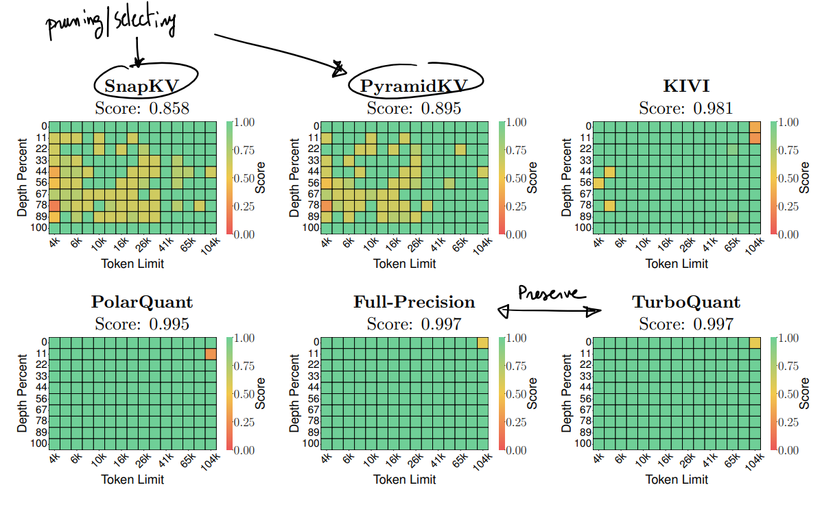
TQ (score: 0.997) is almost identical to Full-Precision (score: 0.997), the uncompressed baseline. Methods like SnapKV (0.858) and KIVI (0.981) that prune or drop tokens lose a lot of accuracy. TurboQuant compresses without pruning, which is why it preserves quality almost perfectly

the chart below compares TQ against Scalar Quantization (SQ) and Binary Quantization (BQ) across real embedding datasets. The X axis is how much you compressed, the Y axis is how much recall you kept. Higher and to the right = better

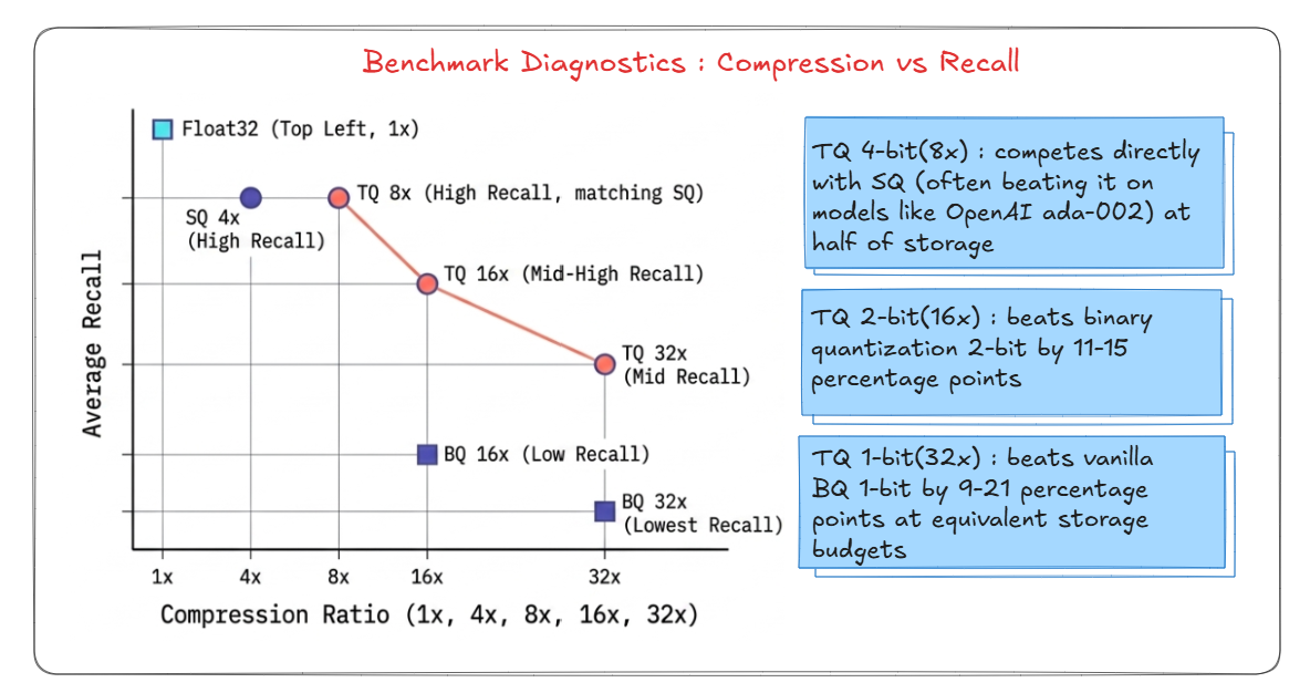
TQ 4-bit (8x compression) matches SQ 4x (which only compresses half as much). TQ 2-bit beats BQ at the same storage. And TQ 1-bit beats vanilla BQ by 9–21 percentage points on recall. Same storage budget, much better results

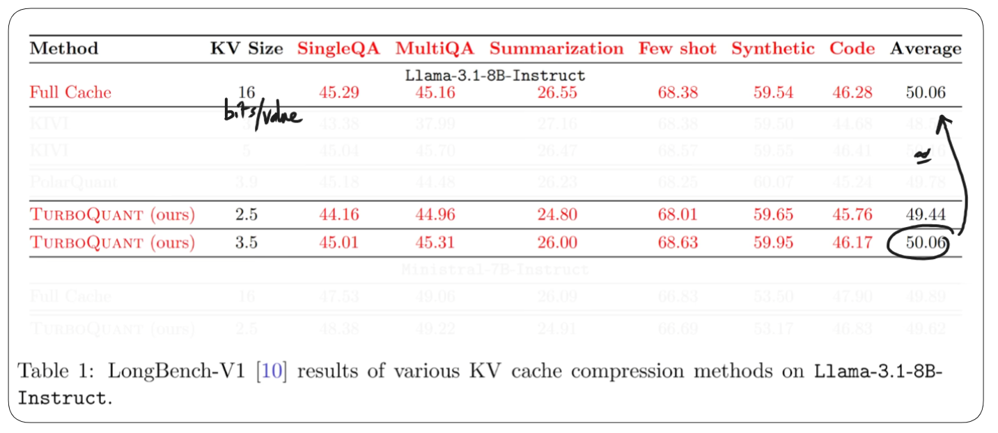
table below [from original paper] shows how TQ performs on a real LLM (Llama 3.1 8B Instruct) using the LongBench benchmark. The KV Size column shows bits per value, lower means more compressed. TQ at 3.5 bits matches the full uncompressed baseline across all task types

Qdrant extensions : the theory to production gap

Qdrant doesn’t just copy-paste the TurboQuant algorithm, it adds 4 real-world fixes that make it actually work on production data. The original paper assumes perfect conditions (isotropic vectors, unit sphere). Real embeddings like OpenAI’s ada-002 or Cohere models don’t behave that way. The 4 extensions below close that gap

1. Length renormalization :

the problem is vanilla MSE quantization systematically shrinks vectors(meaning the quantized vectors end up systematically shorter than original vectors), and to solve this Qdrant borrows the 4-byte fix from (RabitQ) by storing one extra per-vector scalar: which is the ratio of the original length to the centroid reconstruction length and during scoring this stored ratio is multiplied back in to scale the vector back to its original length

think of it like this: imagine you took a photo and it came out slightly darker than reality. Instead of retaking the photo, you just note “this photo is 15% too dark” and brighten it when you show it. Qdrant does the same, it stores how much the vector shrank, then corrects it at search time. Just 4 extra bytes per vector

2. Per-coordinate calibration( anisotropy compensation) :

the original algorithm mathematically assumes that vectors are evenly distributed (isotropic: vectors that are uniformly distributed in all direction evenly across the hypersphere) but real world anisotropic embeddings have high variance directions that can drift off the fixed codebook. qdrant runs a pre-pass on each segment to estimate a (shift, scale) pair per coordinate. this pulls the empirical distribution back onto the codebook’s grid ensuring data isn’t lost

3. support for L2 and unnormalized dot products:

Vanilla TurboQuant assumes all inputs live on the unit sphere, meaning it only naturally supports cosine distance. Qdrant extended the scoring mechanism to unlock L2 and unnormalized dot products by storing the original L2 norm of the vector and mathematically applying it back during the scoring phase.

4. SIMD Acceleration:

to optimize the asymmetric scoring path (the “hot path” of every search), Qdrant built highly optimized integer-arithmetic SIMD kernels. For 4-bit and 2-bit quantization, they map the codebook to an 8-bit lookup table that fits perfectly into a single SIMD register, allowing fast pshufb and maddubs loops. For 1-bit quantization, they implemented RaBitQ’s bit-plane scoring

SIMD (single instruction, multiple data) this is a hardware capability in modern CPUs that allows a single instruction to perform the exact same calculation on multiple data points simultanously

Qdrant implementation

here’s what enabling TurboQuant actually looks like in Qdrant, two collections, same data, one line of difference

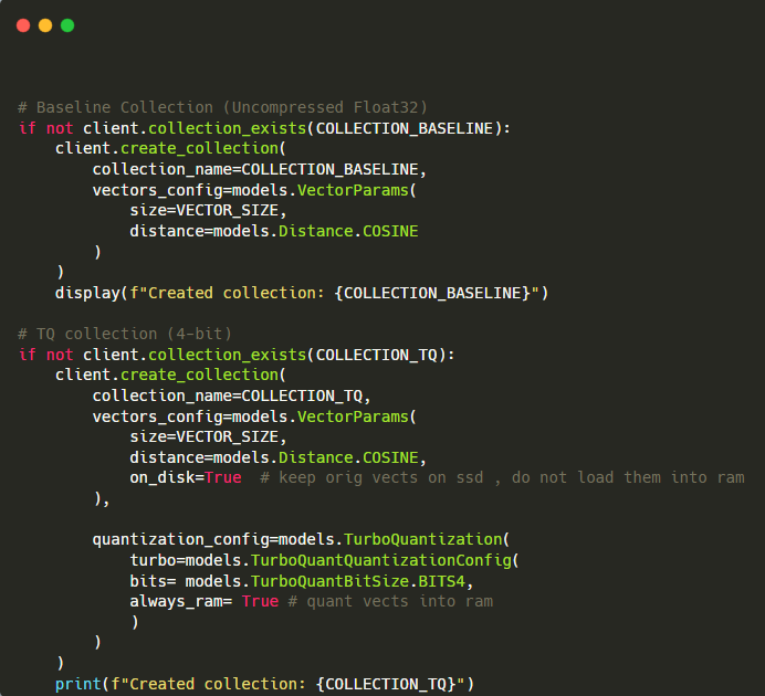
The code above creates two collections side by side. The baseline is plain Float32, full precision, full memory. The TQ collection uses 4-bit TQ with always_ram=True, which means the compressed vectors stay in RAM for fast access while the originals are kept on disk. With this setup you get 8x less RAM usage with almost no recall loss. The on_disk=True flag is the key, original vectors go to SSD, quantized vectors stay in memory

Baseline VS TQ collection

[Image below]Memory footprint comparison: Baseline (Left) vs. TurboQuant (Right). TurboQuant keeps the original ‘source of truth’ vectors on your SSD (via on_disk=True) while pinning only the tiny quantized data in RAM, resulting in a much lighter memory footprint without losing search speed.

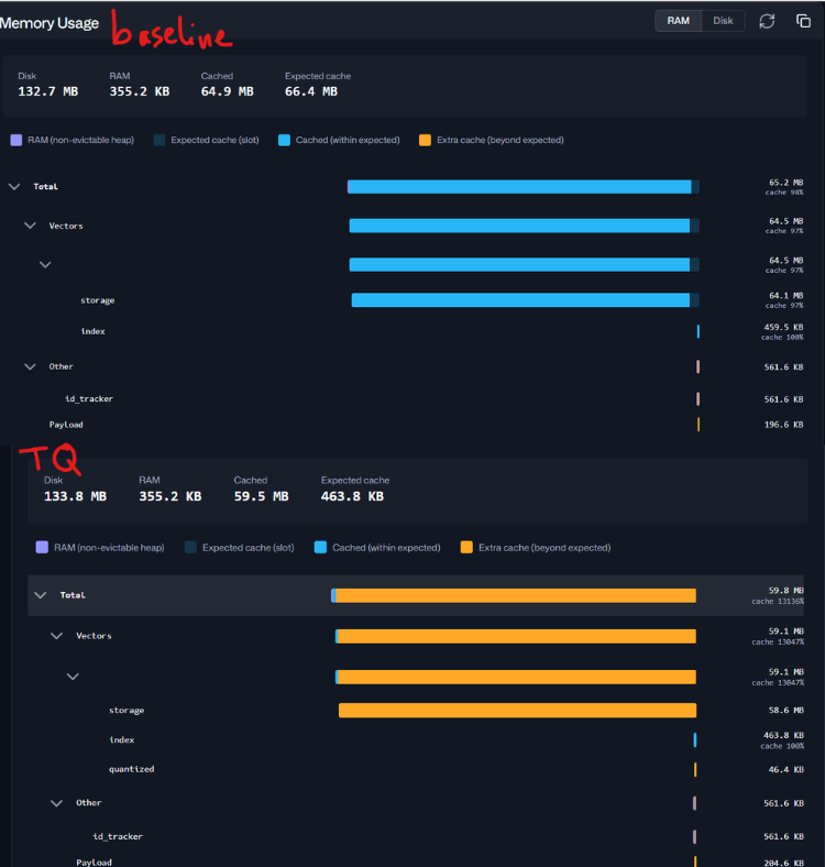
Baseline versus TurboQuant memory footprint

If you notice your dashboard showing higher-than-expected memory usage, remember that the OS is often being ‘helpful.’ When you store original vectors on an SSD, the operating system will automatically keep a copy of those files in spare RAM to speed up future reads. This is not a memory leak! The ‘orange’ bar in your memory dashboard represents the ‘Expected Cache’ that Qdrant needs to stay fast, while the ‘blue’ bar is the OS using leftover RAM for extra speed. You can safely rely on on_disk=True for your original vectors to keep your footprint lean, while using always_ram=True to keep the quantized data lightning-fast.

definitions

pshufb: This is a specific Intel SIMD instruction (_mm_shuffle_epi8). Qdrant uses it as a clever hack to perform “parallel indexing into a 16-byte table,” allowing the CPU to instantly look up multiple quantized values from the codebook in a single clock cycle.
maddubs: This is another SIMD instruction (_mm_maddubs_epi16). It multiplies pairs of 8-bit integers and immediately adds adjacent pairs together. In TurboQuant, this handles the core multiplication step of the dot product between the compressed vector and the query.
lloyd-max algorithm: computes exact optimal centroids to minimize Mean squared error MSE independent of coordinate interactions
Hadamard Transform: A fast mathematical rotation that spreads a vector’s energy evenly across all coordinates. It’s the key that makes TurboQuant’s fixed codebook work on any data distribution without training.

Conclusion

TQ is what happens when the math actually catches up to the engineering problem. For years, the options were either compress aggressively and lose accuracy, or keep accuracy and pay the full memory cost. TQ breaks that tradeoff. The three-step pipeline, rotate, quantize, correct, is elegant because it doesn’t need your data to train on. It works on day one, on any embedding model, at any scale. Qdrant’s four extensions (length renormalization, anisotropy compensation, L2 support, and SIMD acceleration) then take that theory and make it survive contact with real production traffic. 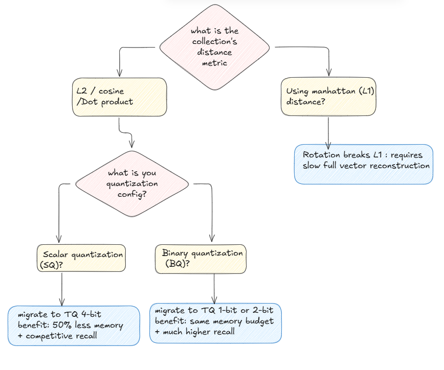The practical takeaway is simple: if you’re running Scalar Quantization today, switching to TQ 4-bit cuts your memory in half with almost no recall hit. If you’re on Binary Quantization, TQ 2-bit or 1-bit gives you the same storage at meaningfully higher recall. It’s a config change, not a re-architecture

References :

Share this article:

(END)